0 Preface
The DDS (Direct Digital Frequency Synthesis) frequency synthesizer can easily output arbitrary waveforms, and the square wave is one of the most commonly used waveforms, and has its particularity. However, the apparent square phenomenon of the output square wave directly affects the quality of the square wave.
1 Reasons for square wave ghosting
Assuming the system clock frequency is 200 MHz, taking the output 3 MHz square wave as an example, the results observed from the analog oscilloscope are shown in Figure 1.
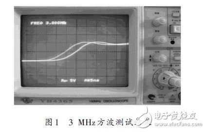
There is a significant double-edge phenomenon in Figure 1, and the spacing between the two rising edges is 5 ns, which is exactly equal to the period of the system clock. This phenomenon can be called square wave ghosting.
According to the working principle of DDS, the phase sequence has periodicity.
During one cycle of the phase sequence, the phase accumulator overflows several times and the amount of residue after each overflow is different. When the residual amount is large enough, the number of accumulations required for the overflow to occur again is reduced once. The decrease in the number of accumulations means that the period of the square wave becomes smaller. When square waves of different periods are superimposed, ghosting occurs.
Using Matlab to simulate the process of DDS to generate a square wave, you can get a more intuitive understanding, as shown in Figure 2.
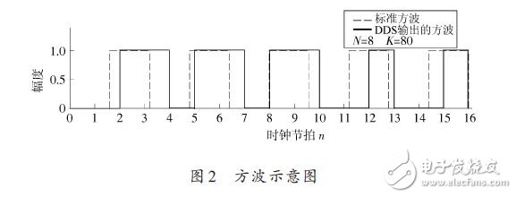
According to the parameter setting in Figure 2, the period of the square wave is equal to:
As can be seen from Figure 2, in order to output a square wave with a period of 3.2Tc, the actual output of the DDS frequency synthesizer in one cycle of the phase sequence is: a square wave with a period of 4Tc and a duty cycle of 50%, two A square wave with a period of 3Tc and a duty ratio of 75%, and a square wave with a period of 2Tc and a duty ratio of 25%. In the average sense, it is just a square wave with a period of 3.2Tc and a duty cycle of 50%. Therefore, the square wave output from the DDS frequency synthesizer not only fluctuates in cycles, but also the duty cycle fluctuates.
If the DDS frequency synthesizer is viewed as a component frequency, the following conclusion can be drawn under the condition that the Nyquist sampling theorem [4] is satisfied: when a continuous signal such as a sine wave is output, the DDS can achieve an arbitrary ratio of frequency division; When a square wave or the like has a signal with a transition edge, the period of such a signal can only be an integral multiple of the system clock period, otherwise a ghosting occurs.
2 Research and implementation of square wave improved algorithm
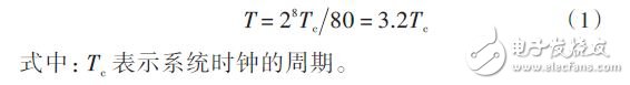
In order to solve the square wave ghosting problem, it can be analyzed from the perspective of time domain. A plurality of square waves of different periods are superimposed together, and a schematic diagram is shown in FIG. 3.
In Figure 3, the a point and the d point are dithered downward, so that the b point and the c point are shaken upward, and the square wave ghosting can be effectively weakened after multiple superpositions, or even completely eliminated. However, how to accurately judge the four points a, b, c, and d becomes the biggest obstacle to achieve this method.
Looking closely at Figure 3 and Figure 2, by introducing the concept of clock beats, we can find four points based on the judgments a, b, c, and d. First, define the period and rising edge of the square wave. Take the 50% duty cycle as an example. These two values ​​can be expressed as:
Among them, ceil means rounding in the positive infinity direction, and floor means rounding in the negative infinity direction, all of which are Matlab operators [5].
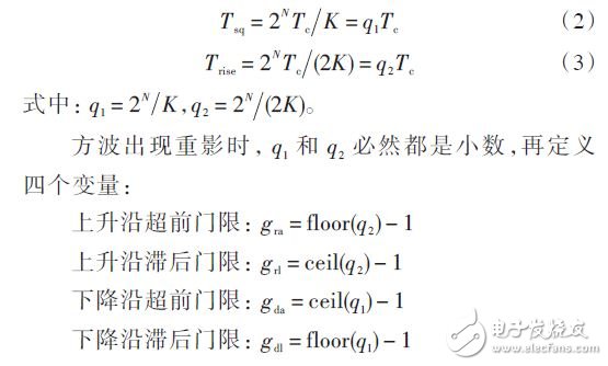
When the frequency of the system clock is 200 MHz, the output 3 MHz square wave is taken as an example. The calculation results are shown in Table 1.
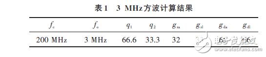
Similar to Figure 3, a schematic diagram of a 3 MHz square wave is shown in Figure 4.
As can be seen from Fig. 4, points a and b occur at a position where the clock tempo is 33, and points c and d occur at a position where the clock tempo is 65. When c point appears, it means that the period of this square wave is small. The next clock section according to the law of Fig. 3, using the high and low level information of the original square wave signal at the position where the clock beat is grl and gda. Obtain four points a, b, c, and d. Assuming that the number of bits in the DAC is 14 bits, the implementation of the square wave improvement algorithm can be divided into the following three steps:
In the first step, a counter is defined and the carry output signal of the phase accumulator is used as the clear signal, that is, the counter is cleared once every time the phase accumulator overflows. Therefore, the count value of this counter indicates the clock tick in Fig. 4.
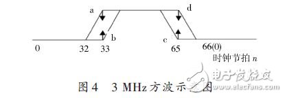
In the second step, a state machine is defined, assuming that the counter has a count value of num, and the simplified state transition diagram is as shown in FIG.
The clock ticks of the state RISE tag are grl. In this state, if the original square wave signal is high, a point is obtained; if the original square wave signal is low, b point is obtained. The clock tempo of the state DOWN flag is gda. In this state, if the original square wave signal is low, c point is obtained; if the original square wave signal is high level, d point is obtained.
The third step is to define a random variable random, which varies from 0 to 2 048 and can be implemented by an 11-bit m-sequence. Using the verilog language bit splicing operator [6], the data sent to the DAC at points a and d is defined as 10 240 plus random, ie "{3'b101, random}"; will be sent at points b and c The data for the DAC is defined as 4 096 plus random, which is "{3'b010, random}".
3 Testing and summary
After using the new square wave algorithm, the test results are shown in Figure 6.
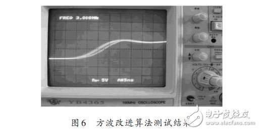
Comparing Figure 6 with Figure 1, it can be seen that the width of the square wave ghost is shortened from 5 ns to 3 ns, and the rising edge is solid and no longer consists of two edges.
On the other hand, in Fig. 6 and Fig. 1, the rise time of the square wave is about 15 ns, which indicates that the square wave improvement algorithm does not cause an increase in the rise time.
Guangzhou Bolei Electronic Technology Co., Ltd. , https://www.nzpal.com